Plotting the exponential function

This example demonstrates how to import a local module and how images are stacked when two plots are created in one code block (see the Force plots to be displayed on separate lines example for information on controlling this behaviour). The variable N from the example ‘Local module’ (file local_module.py) is imported in the code below. Further, note that when there is only one code block in an example, the output appears before the code block.

• 
• 

# Code source: Óscar Nájera
# License: BSD 3 clause

import matplotlib.pyplot as plt
import numpy as np

# You can use modules local to the example being run, here we import
# N from local_module
from local_module import N  # = 100


def main():
    """Plot exponential functions."""
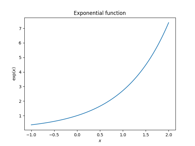
    x = np.linspace(-1, 2, N)
    y = np.exp(x)

    plt.figure()
    plt.plot(x, y)
    plt.xlabel("$x$")
    plt.ylabel(r"$\exp(x)$")
    plt.title("Exponential function")

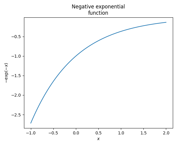
    plt.figure()
    plt.plot(x, -np.exp(-x))
    plt.xlabel("$x$")
    plt.ylabel(r"$-\exp(-x)$")
    plt.title("Negative exponential\nfunction")
    # To avoid matplotlib text output
    plt.show()


if __name__ == "__main__":
    main()

Estimated memory usage: 193 MB